Subset selection for climate prediction

The Goal

Global climate models are useful tools to predict what the climate might look like decades into the future. However, as the figure above shows, projections of global land-surface temperatures vary between 21 current generation climate models. So which model’s projections are the most “correct”? Of course we cannot be sure because we don’t have observations of the future. But we can reduce the chances of biased projections by carefully weighting or subselecting models in the observed historical period. In this blog post I discuss two methods: a machine learning approach and a combinatorial optimisation approach, both which can improve prediction accuracy in climate projections.

Model-as-Truth

We will optimise for the Root Mean Squared Error (RMSE) between two 2-dimensional (latitude vs longitude) climatological (average over 30-years of temperature data) arrays. Because we have no observations of the future, one way to test whether our approach is working is to select one of the 21 models shown above, as the “truth” (i.e. response variable). We then fit a statistical model using all other climate models as the features (also known the predictor, explanatory, or independent variables) to explain the response. We finally test the trained statistical model to predict unseen projections of temperature data (the test set) from the same model-as-truth. Testing the performance of the statistical model on unseen data is a simple and effective way to test for overfitting (when the model follows the data points too closely and does not generalise on unseen data).

The Lasso

The Lasso is one of the most simple statistical learning approaches that minimises the quantity:

The first term is the residual sum of squares as in the well known least squares regression. This term finds coefficients that fit the data well. The second term is a shrinkage penalty, keeping the sum of the coefficients low. The tuning parameter serves to control the relative impact of the two terms on the regression coefficients. When is large the coefficients approach zero (reducing variance but increasing bias), when it is small the coefficients will be similar to least squares regression (reducing bias but increasing variance). This bias-variance trade-off forms the basis of many machine learning models. One key feature of the Lasso is that the final model is sparse meaning many of the coefficients will be shrunk to exactly zero, so we will end up with a subset of size K from the initial P simulations. This subset selection quality (also known as the penalty) is why we will use the Lasso, as we then depend on fewer climate models to make predictions.

A Simple Example

Here we select one climate model as the “truth”, say EC-EARTH (grey line in figure above). We train the Lasso on the 1941-1970 temperature climatology, where each grid cell is one of n (602 in this case) samples, and each of the remaining P (20 in this case) models is a feature. After tuning the hyperparameter using 3-fold cross validation, coefficients for 13 of the 20 models are shrunk to zero, and the remaining 7 coefficients take on continuous values. The RMSE on the training set between the response and the subset is 0.8. Had we simply used the arithmetic mean of the 20 runs, known as the multi-model mean “MMM” which is typically used in climate science, we would have gotten a RMSE of 1.92. So the Lasso is giving us a 58% (1.92-0.8/1.92)*100 improvement over the naive approach!

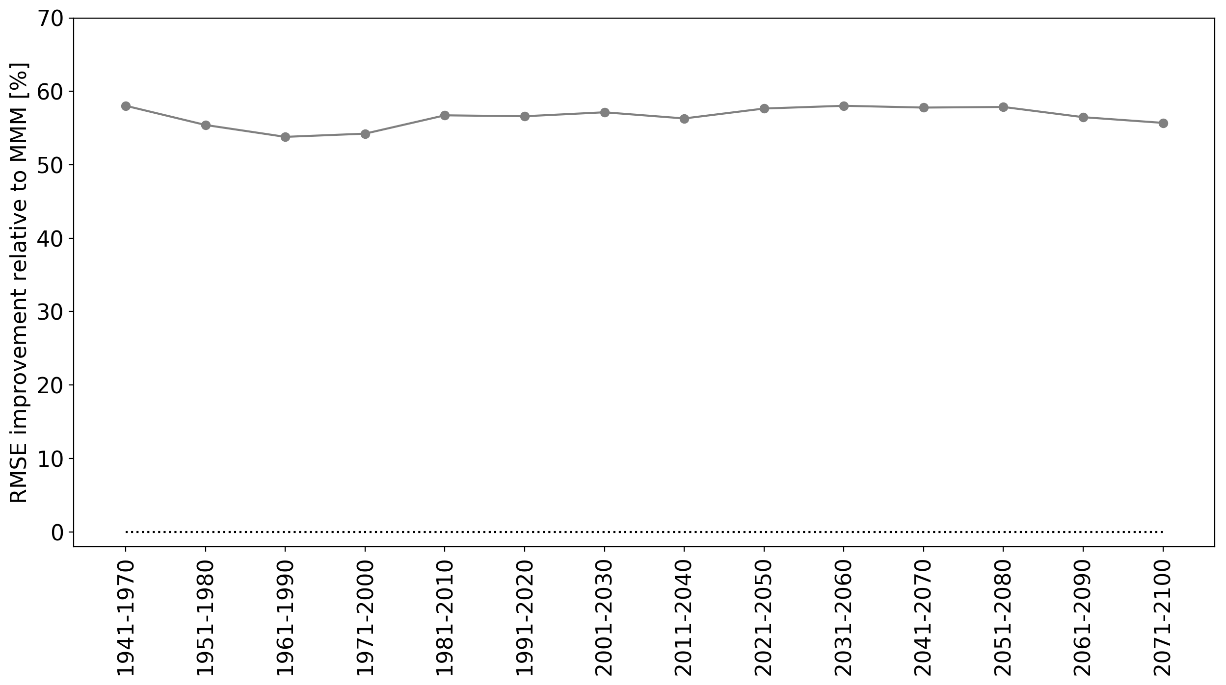
However, of course our statistical model will perform well in-sample in the 1941-1970 period, since this is the data that was used to train the model. To really understand how well it is performing, we must test it on unseen data. The figure below shows the RMSE for 30-year climatologies for 1941-1970 (in-sample) and all remaining 30-year periods until the end of the 21st century (out-of-sample).

The results are impressive. The RMSE remains fairly low until the end of the 21st century. The figure below shows the percentage improvement over the MMM. One would expect predictability to slowly decrease the further we go from the training set, but the line is impressively flat. Since Lasso is one of the least flexible machine learning approaches (it results in a sparse linear solution), it is less prone to overfitting than many other machine learning methods.

Each Model as Truth

Perhaps we got lucky? We can rotate through each of the 21 models, and use each as the “truth” (i.e. response variable), training on the 1941-1970 climatology and testing until the end of the 21st century. We now result in 21 lines showing prediction skill relative to the MMM:

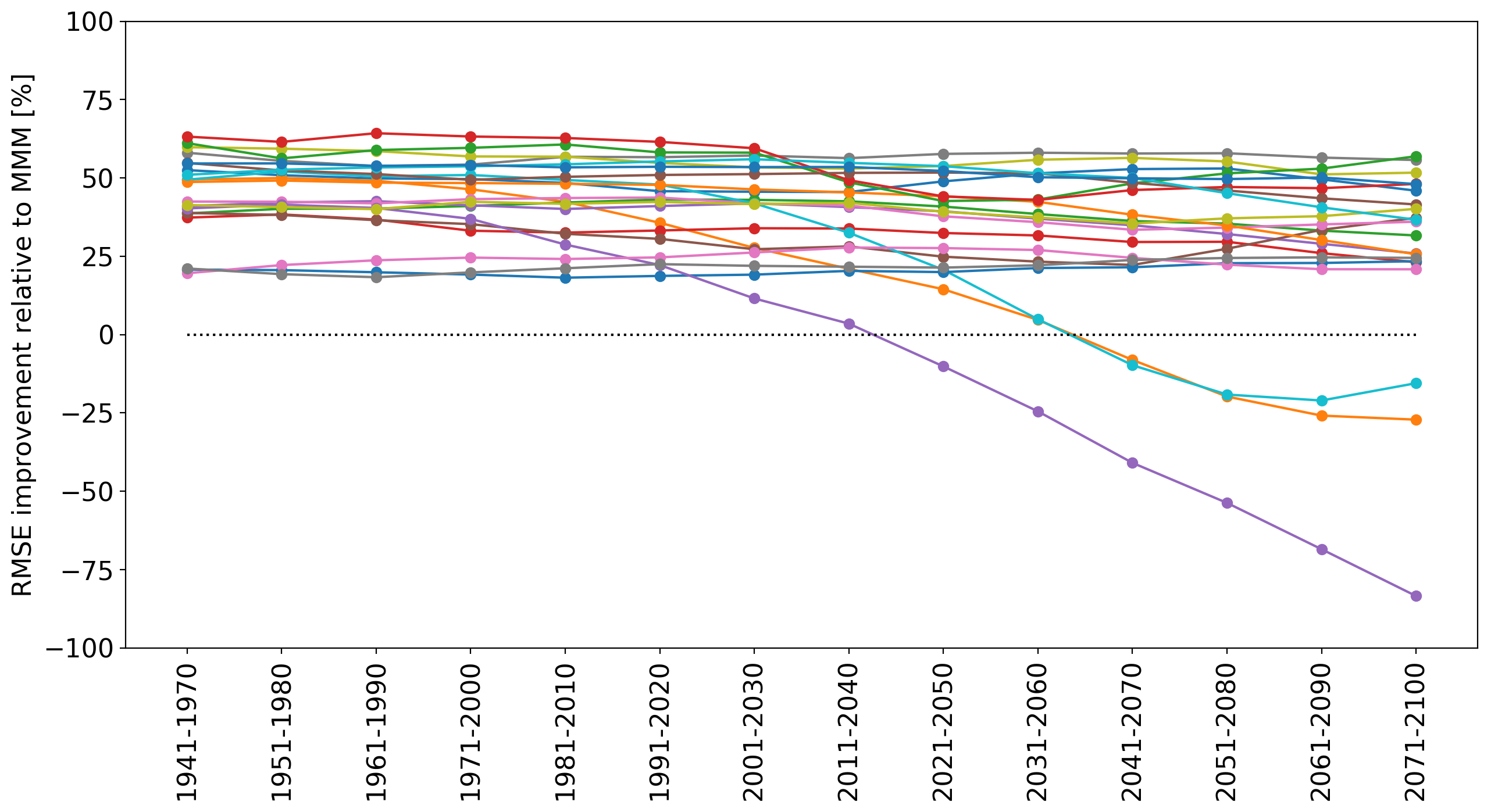
We now see that it is difficult to predict end of century climatologies for 3 of the 21 models. Perhaps there is some non-linear response to greenhouse-gas forcing that the statistical model could not detect in the 1941-1970 period. However, overall, temperature in 18 of the models can be predicted until the end of the century with much greater accuracy than using the MMM.

Non-convex Optimisation

The penalty in the Lasso means it is a convex optimisation problem. This is a helpful setting because it can be solved iteratively and quickly with coordinate descent. But what if we want our coefficients to be discrete, i.e. take on values of either 0 (the climate model is disregarded) or 1 (the climate model is kept)? This is known as a non-convex () or an NP-hard problem. The travelling salesman problem is a well known NP-hard problem. Such problems can be solved via brute force. In the case of the problem discussed in this post, we can try every possible combination of climate models from subset size K = 1..P, and in the end use the combination whose arithmetic mean gives us the lowest RMSE compared to the model-as-truth. This would be extremely computationally expensive though, since there are possible combinations.

Using Gurobi to Solve our Problem

Gurobi is a proprietary (but free for academics) software that uses branch and bound algorithms to solve combinatorial optimisation problems. The problem we are dealing with here is specifically a mixed integer quadratic programming (MIQP) problem because the decisions are binary and the cost function is quadratic from the “squared error” in RMSE.

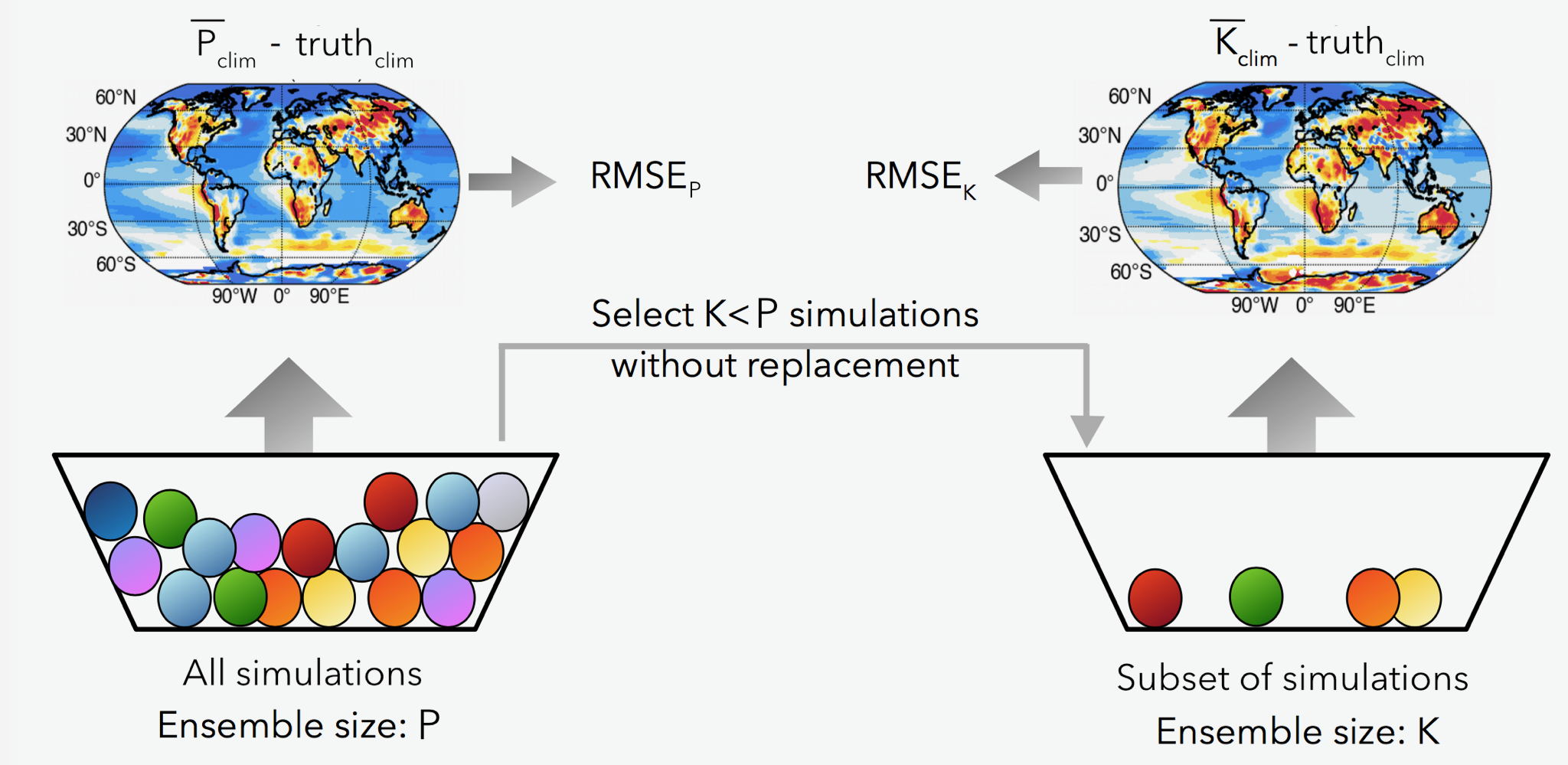
The schematic below describes what we want: a subset of size K, for which the RMSE between and the “truth” is minimised. Because the weights can only take on 0 or 1, the final solution is even more interpretable than the Lasso. The schematic would be similar for the Lasso, except one would take a weighted mean of the subset based on the coefficient values and not an equally weighted mean of the subset.

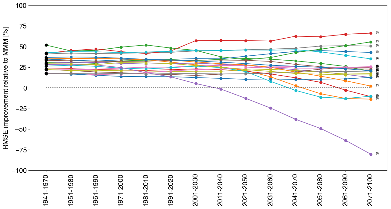
The following figure shows the RMSE improvement over the MMM, for each model-as-truth, but this time using Gurobi. The number of models K selected by Gurobi for each model-as-truth is shown in small font beside each line. The subset size K that resulted in the lowest training RMSE, was used to make predictions. As with the Lasso, we see breakdown in predictability for similar models, except now we have a completely different type of solution! The improvement relative to the MMM is slightly less than for the Lasso, since the weights are restricted to being binary.

Once we are happy with the performance using this model-as-truth setup, we can use real observations of the world as our “truth”. Of course since we don’t have real observations beyond the current year, we can only train the statistical model without testing out-of-sample performance until the end of the 21st century. The best we can do is to make predictions and hope they are accurate. However model-as-truth experiments serve as a very good proxy for predictive skill. If you want to know more about using Gurobi or model-as-truth experiments, read Herger, 2018

Thanks for reading. If you have any questions, don’t hesitate to ask in the comment box below.