The bias-variance tradeoff « Oliver Angelil

Prelude

A key concept in supervised statistical learning / machine learning is the bias-variance tradeoff (also known as the accuracy-precision tradeoff). This is an optimisation problem where these two properties compete against each other. Let us begin with the ordinary least squares regression approach, which only tries to reduce bias:

$\sum_{i=1}^{n}\Bigg(y_{i}-\beta_{0}-\sum_{j=1}^{P}\beta_{j}x_{ij}\Bigg)^{2}$

This approach may suffice when n » p (many more samples than predictors). A rough rule of thumb is that at least 10 times more samples than predictor variables are needed to prevent overfitting (when the model follows the data too closely and cannot generalise). However the ordinary least squares approach becomes an issue when the number of predictors increases or the number of samples decreases. In these cases, bias can still be reduced: the trained statistical model can fit the data extremely well. Unfortunately learning the data too well results in overfitting. A clear sign of overfitting is when a model performs well on training data, but cannot generalise and therefore performs poorly on unseen test data. We say that the model is too complex, and therefore we need to seek out a more simple model.

Ridge Regression

Ridge regression is one of the most basic statistical learning methods that can reduce the complexity of a model and therefore reduce the chance of overfitting. Ridge regression minimises the quantity:

$\sum_{i=1}^{n}\Bigg(y_{i}-\beta_{0}-\sum_{j=1}^{P}\beta_{j}x_{ij}\Bigg)^{2} + \lambda\sum_{j=1}^{P}\beta^2_{j}$

Note this is least squares regression but with an additional shrinkage term. The tuning parameter $\lambda$ serves to control the relative impact of the terms in the equation above on the regression coefficients. When $\lambda$ is large the coefficients (betas) approach zero (reducing variance but increasing bias), when it is small the coefficients will be similar to least squares regression (reducing bias but increasing variance).

A simple example

The code for this example can be found in my github repo. Suppose I have 200 predictor variables, each with 1000 samples. I want to predict a continuous response variable. We first split the data up into training and test sets (a 60/40 ratio is typical). I loop through a list of $\lambda$ , for each $\lambda$ I fit ridge regression to the training data, then calculate the MSE on the training and test sets. I am ultimately aiming to get the lowest possible error on the test set. This figure shows the functional relationship between lambda and MSE:

time_series

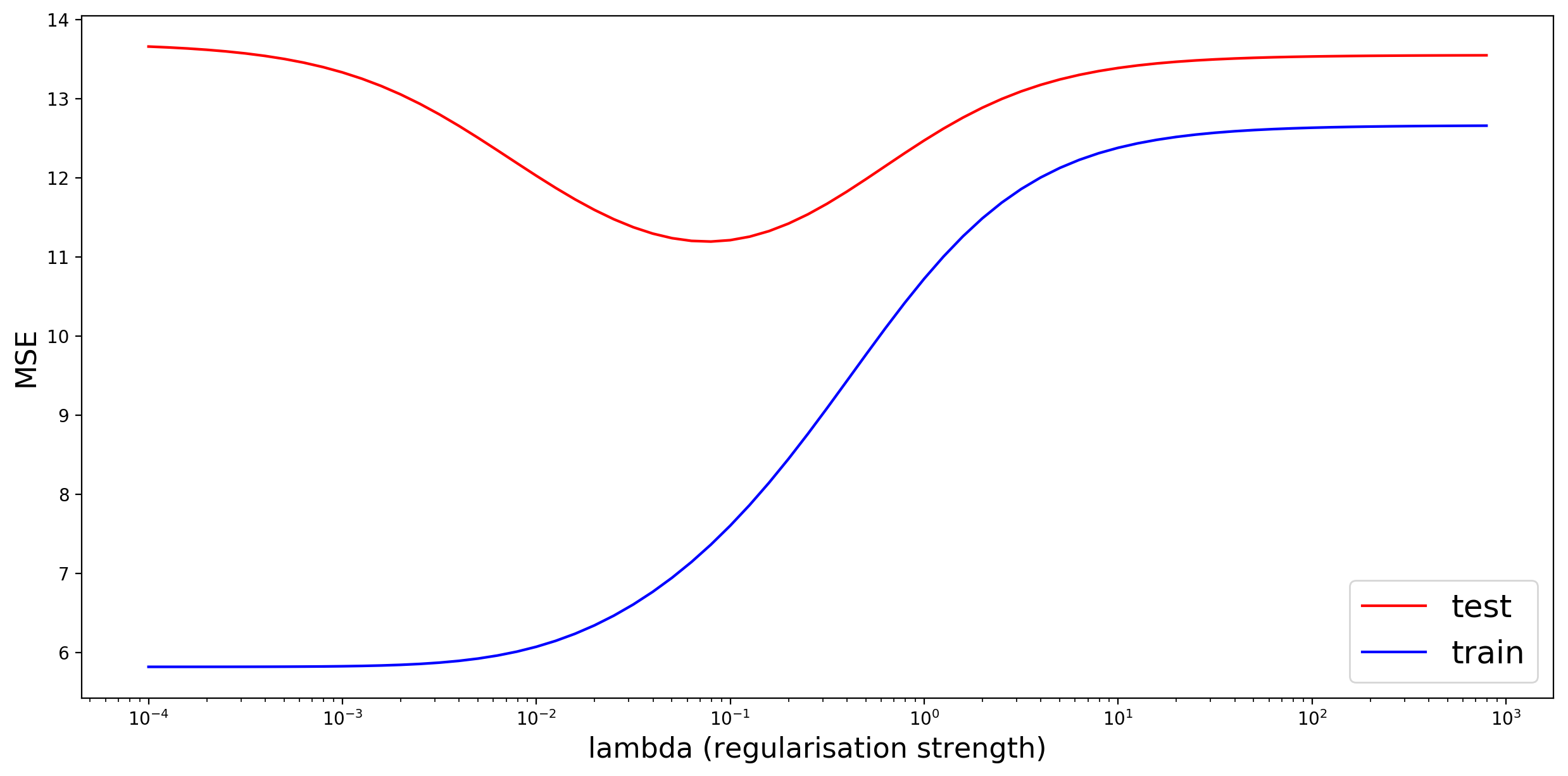
When $\lambda$ is very small (far left), we are essentially fitting an ordinary least squares model. The training error is very low, but the test error is high: a typical case of overfitting! Our model is too complex. As we increase $\lambda$ , the training error increases and the test error decreases. When the test error is at its lowest we have found the sweet spot between bias and variance. As $\lambda$ further increases, the model no longer fits to the data well enough (too little variance), it is “too simple” and underfits the data, and the test error increases again. One can use a number of different machine learning methods (Lasso, Random Forest Regression, Support Vector Regression) for this problem, and this “U” shape will likely result.